September 25, 2021
This was a weekend project I tackled after being captivated by DeepMind's Atari gameplay videos. I'd been wanting to dive into Deep Q-Learning for a while, and LunarLander-v2 seemed like the perfect starting point. The goal: train an agent to land a lunar module and understand how tweaking hyperparameters changes its behaviour.
In traditional reinforcement learning problems with finite, discrete Q-states, you can list all Q-states and store them as an index-value pair or table. The index is the pair (state, action) and the value is the estimated Q-value for that state-action pair.
However, LunarLander-v2 has a continuous state space. You can't tabulate Q-states without transforming the state space.
I used a function approximation approach to solve LunarLander-v2 using Q-learning. The function approximation model I chose is a Neural Network. From the Universal Approximation Theorem, this is a well-justified choice.
LunarLander-v2 is an OpenAI Gym environment that lets you benchmark Reinforcement Learning algorithms. It has a researcher-friendly implementation and you can add custom environments.
The environment state can be accessed through the state vector. Here are the key details:
The LunarLander-v2 is reward engineered. The rewards are dense and shaped! (unlike what Deepmind did with Atari). So, solving this should be a lot easier for RL.
The environment is considered solved when average reward over 100 consecutive episodes exceeds +200. Fuel is infinite, so an agent can learn to fly and land on its first attempt.
I had access to a 4-core MacBook Air 2017 model with 1.6GHz clock speed. My approach was influenced by these hardware constraints.
At first, discretizing states seemed like a good solution. However, the state space becomes too large when we discretize the continuous state space.
There are 8 state variables in the state vector. Assuming we transform each into 30 discrete values, we'd have \(30^8\) states, which is approximately \(6.5 \times 10^{11}\). The number of Q-states \(Q(s,a)\) would be around \(10^{12}\). I concluded this wasn't worth exploring.
Given a sequence of states and actions \(\langle s, a \rangle\) and the corresponding reward \(r\) for landing in state \(s\), we can solve the MDP using Q-learning- an off-policy, model-free learning method. This gives us the value of an action in a particular state. The goal is to maximize total reward.
The core is the Bellman Equation as a value iteration update:
\[ Q^{n}(s_t, a_t) = Q^{n-1}(s_t, a_t) + \alpha (r_t + \gamma \max_a Q^{n}(s_{t+1}, a) - Q^{n-1}(s_t, a_t)) \]
This works when Q-states are finite, discrete, and tractable. For continuous state spaces, we need function approximation methods. I chose a Neural Network.
We replace \(Q(s,a)\) with \(Q(s,a,\theta)\) where \(\theta\) represents the neural network weight parameters.
When Q-learning converges, the temporal difference error \((r_t + \gamma \max_a Q^{n}(s_{t+1}, a) - Q^{n-1}(s_t, a_t))\) goes to zero. This is our goal, so we can use it to write the cost function:
\[ \text{cost} = (Q(s, a, \theta) - (r(s, a) + \gamma \max_a Q(s', a, \theta)))^2 \]
This is just Mean Squared Error between target and prediction. The current Q-value is the prediction; immediate and future rewards are the target.
Architecture 1 (shown below) seems valid at first. The network receives state and action as inputs and outputs a Q-value.
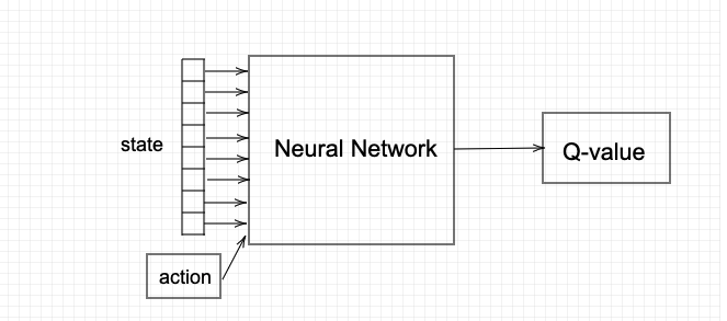
However, this is inefficient from a technical standpoint. Since the cost function requires the maximum of the next Q-state value, we'd need several network predictions for a single cost calculation.
Instead, I used Architecture 2:
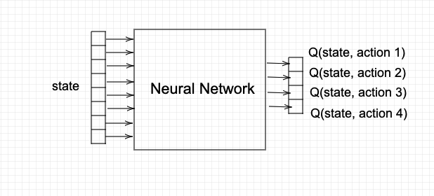
In the cost function, the target is \(r(s,a) + \gamma \max_a Q(s',a,\theta)\). This target changes continuously with each step in the environment, leading to unstable training. You're chasing a moving target.
To fix the target for some iterations and control parameter updates, I used two Deep Q-networks:
This leads to more stable training. The cost becomes:
\[ \text{cost} = (Q_{\text{prediction}}(s, a, \theta) - (r(s, a) + \gamma \max_a Q_{\text{target}}(s', a, \theta)))^2 \]
When you run Q-learning on state-action pairs as they occur during simulation, the data is highly correlated. Sequential actions are correlated with each other and not randomly shuffled. This causes Catastrophic Forgetting- the network unlearns things it learned earlier.
Neural networks converge better when data is independent and identically distributed. This ensures enough diversity in training data for the network to learn meaningful weights that generalize well.
The solution: store experiences in a large array. During training, randomly sample from this experience replay data to train the neural network. In practice, the maximum size of experience replay memory is limited.
The Deep Q-Learning architecture has two neural networks (Prediction and Target) plus Experience Replay Memory for storing training data.

The DQN trains over multiple timesteps across many episodes. Each timestep follows this sequence:
Experience Replay selects an \(\epsilon\)-greedy action from the current state, executes it in the environment, and receives a reward and next state.
All prior observations are saved as training data. Then I randomly select a batch of samples from this training data, so it contains a mix of older and recent samples.
This batch is inputted to both networks. The Prediction Network takes the current state and action from each sample and predicts the Q-value for that action. This is the "Predicted Q-Value."
The Target Network takes the next state from sampled data to predict the best Q-value out of all actions that can be taken from that state. This is the "Target Q-Value."
The Predicted Q-Value, Target Q-Value, and observed reward are used to compute the loss to train the Prediction Network. The Target Network is not trained. The weights of the Target Network are copied from the Prediction Network after every episode ends, not within every step.
This repeats until the environment is solved.
I decoupled experience replay sampling from generating experience using \(\epsilon\)-greedy policy. This is slightly different from standard implementations where sampling happens when taking steps in the environment. Theoretically, there's no difference in results. However, this architecture works better for larger-scale distributed RL problems and makes adding methods like prioritized experience replay easier.
Additionally, the greedy policy is evaluated every 500 episodes. If performance is satisfactory, training stops.
The complete training algorithm is detailed below:
replayMemoryreplayMemoryreplayMemoryThe algorithm details the training procedure. I have decoupled experience replay sampling from generating experience using \(\epsilon\)-greedy policy. This is slightly different from what's in literature, as sampling of experience replay is not done when taking a step in the environment. Theoretically, there's no difference in results.
However, I feel this is a better way to architect the process that will help in larger-scale RL problems requiring distributed RL. This decoupling makes adding and testing methods from literature related to experience sampling easier (e.g., Prioritized Experience Replay).
Additionally, the greedy policy that is learned is evaluated every 500 episodes. If performance is satisfactory, training stops.
The trained agent uses these parameters:
| Parameter | \(\gamma\) | Initial \(\epsilon\) | \(\epsilon\)-decay | \(\omega\) | LR |
|---|---|---|---|---|---|
| Values | 0.7 | 1.0 | 0.99975 | 0.001 | 0.0001 |
Neural Network Architecture: A two hidden-layer architecture.
| Input Layer | Hidden Layer 1 | Hidden Layer 2 | Output Layer |
|---|---|---|---|
| 8 | 64 | 16 | 4 |
The reward for each training episode, the 100-episode moving average, and test performance are shown below.
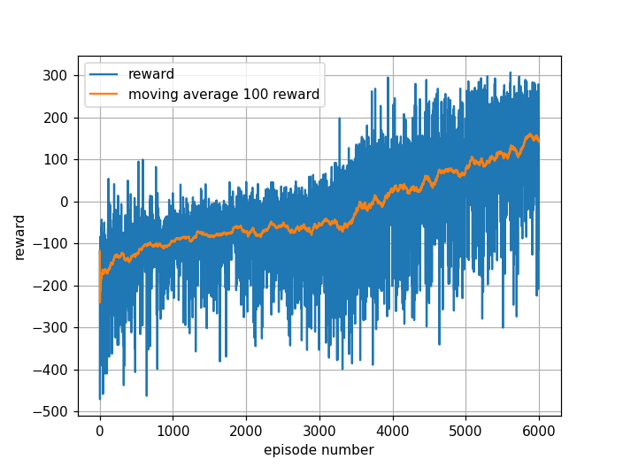
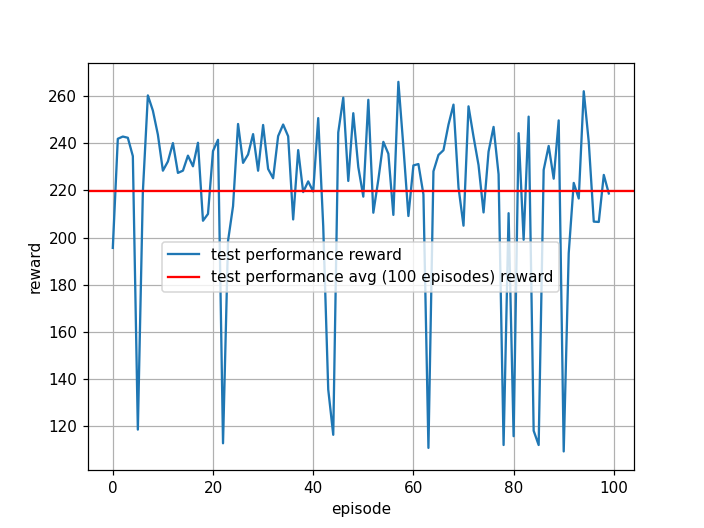
For the trained agent, the moving average reward during training gradually increases and the agent learns to land. The test performance over 100 consecutive episodes gives an average reward of 219. This clearly beats the benchmark (+200) for solving LunarLander-v2.
Note: All figures show 100-point moving averages instead of actual rewards, since raw rewards are too noisy to interpret easily.
Results with 0.25, 0.5, and 0.99 for \(\gamma\) are shown below.
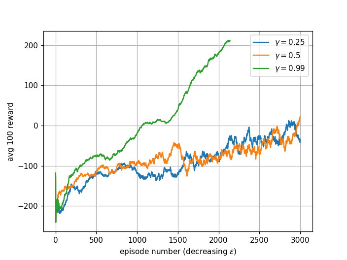
A larger discount factor treats distant future rewards closer to immediate rewards. A smaller discount factor favors immediate rewards and maximizes short-term gain.
\(\gamma = 0.25\): This small discount factor makes the agent short-sighted. Initially, the agent learns to avoid the bottom half of the screen and flies off the top, trying to avoid potential crashes. Due to low \(\epsilon\)-decay, it eventually figures out landing. However, it wobbles a lot before landing, increasing crash probability. The agent fails to solve the environment within 2000 episodes.
\(\gamma = 0.5\): Produces similar behaviour to \(\gamma = 0.25\). Both values aren't large enough for the agent to learn landing within 2000 episodes. The agent takes actions that are best short-term but isn't far-sighted enough. It would eventually solve the environment after arbitrarily many episodes since Q-learning is off-policy and Q-values converge to optimal values with non-zero exploration.
\(\gamma = 0.99\): The best value. Large enough for the agent to be far-sighted and consider rewards many timesteps ahead. It converges to the optimal policy much faster than other values.
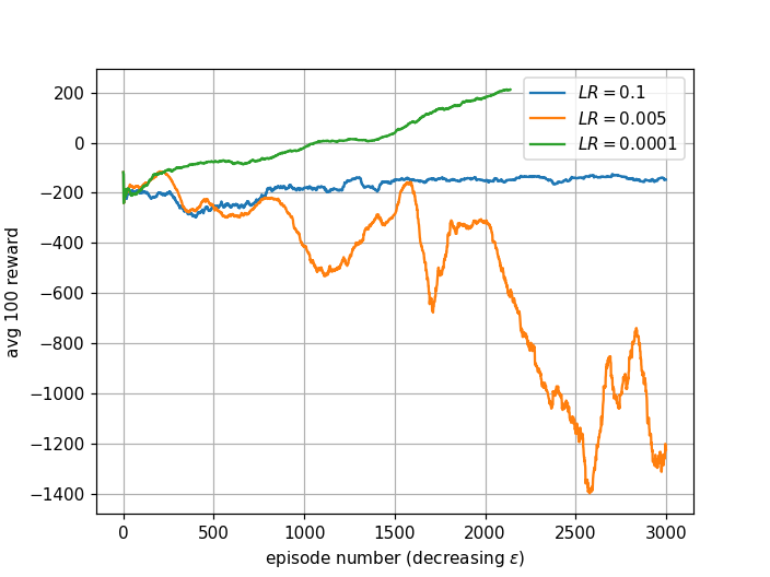
Learning rate decides how much the weights update in each pass toward minimizing cost. Too small makes learning slow and difficult to converge. Too large may miss the local optimum and behave like random actions.
LR = 0.005: Average reward drops very low then rises later, but doesn't learn to land within 3000 episodes.
LR = 0.1: Too large. The agent misses the optimum and behaves like a random agent, learning nothing.
LR = 0.0001: Balanced- not too small, not too large. The agent successfully learns to land and solve the environment.
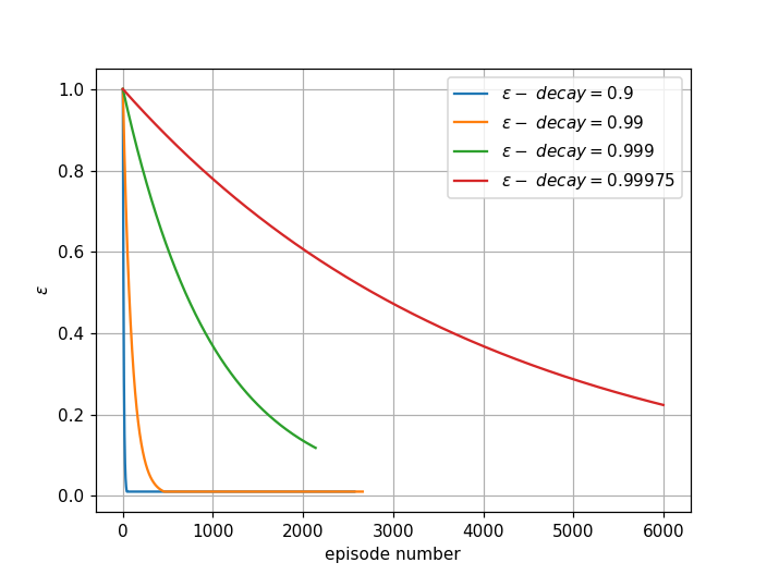
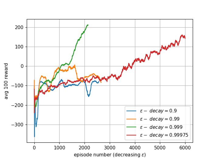
The exploration-exploitation control parameter \(\epsilon\)-decay dictates how fast the agent switches from exploration to exploitation. The first figure shows how fast \(\epsilon\) decays by episode number.
Smaller \(\epsilon\)-decay drops \(\epsilon\) close to zero after very few episodes. This means the agent quickly switches to exploitation with limited knowledge. When \(\epsilon\)-decay = 1.0, the agent always explores and never uses learned experience.
The recommended values (\(\epsilon\)-decay = 0.999 and 0.99975) focus on exploration and learning in early episodes, then slowly switch to exploitation later, generating the best learning results.
In my experiments, since minimum \(\epsilon\) is 0.01, this is sufficient for the agent to converge to optimal Q-values (because \(\epsilon > 0\)) given enough training episodes.
This post details the theoretical foundations of Q-learning and value function approximation, and the implementation of Deep Q-Network (DQN) algorithm for solving the lunar lander problem.
In another post (Part-2), I plan to explore prioritized experience replay. Uniform sampling is a potential limitation of the current framework. I also intend to explore other advanced algorithms like Dueling DQN and policy gradient methods.
It is probably worth it to also use a different NN architecture like CNNs to understand in the magnitude of iumprovement in performance.